Case 04 / Safety
What safety signals emerge?
Which treatment-emergent adverse events were recorded, by system organ class and preferred term?
Precomputed results · R and Python executed locally · no browser analysis engine
Executed source code
Current-view SVG rendering: TypeScript figure source and display controller. These render existing results; they do not run the R/Python analysis.
Full seven-case analysis pipeline. The exact executed file; use the commands below. This code is read-only.
# Clinical Data Lab: independently executed R analysis of CDISC Pilot XPT.
# Run: Rscript --vanilla analyze.R INPUT_DIRECTORY OUTPUT_DIRECTORY
# Packages must already be installed. No network or installation at runtime.
library(haven)
library(jsonlite)
library(survival)
args <- commandArgs(trailingOnly=TRUE)
input <- args[1]; output <- args[2]
dir.create(output, recursive=TRUE, showWarnings=FALSE)
read <- function(name) {
  x <- as.data.frame(read_xpt(file.path(input, paste0(name, '.xpt'))))
  x[] <- lapply(x, function(v) {if(is.character(v)) {v[is.na(v)] <- ''; trimws(v)} else v})
  x
}
stats <- function(x) {
  x <- x[!is.na(x)]; n <- length(x)
  m <- if(n) mean(x) else NA_real_
  s <- if(n>1) sd(x) else NA_real_
  margin <- if(n>1) qt(.975,n-1)*s/sqrt(n) else NA_real_
  list(n=n,estimate=m,sd=s,lower=m-margin,upper=m+margin)
}
adsl <- read('adsl'); ae <- read('adae'); q <- read('adqsadas'); lab <- read('adlbc'); tte <- read('adtte')
stopifnot(!anyDuplicated(adsl$USUBJID), !anyDuplicated(tte$USUBJID), all(tte$CNSR %in% c(0,1)))
stopifnot(all((adsl$DISCONFL=='Y')==(adsl$DCDECOD!='COMPLETED')))
q <- subset(q, PARAMCD=='ACTOT' & ANL01FL=='Y' & DTYPE=='')
stopifnot(!anyDuplicated(q[c('USUBJID','AVISIT')]))
lab <- subset(lab, PARAMCD=='ALT' & AVISIT=='End of Treatment')
stopifnot(!anyDuplicated(lab$USUBJID))
cases <- c('baseline','disposition','longitudinal','adverse-events','laboratory','subgroups','time-to-event')
out <- setNames(lapply(cases,function(x) list()),cases)
arms <- c('Placebo','Xanomeline Low Dose','Xanomeline High Dose')
terms <- unique(ae[c('AEBODSYS','AEDECOD')]); terms <- terms[order(terms$AEBODSYS,terms$AEDECOD),]
for(stratum in c('All','F','M')) {
  cohort <- if(stratum=='All') adsl else subset(adsl,SEX==stratum)
  for(arm in arms) {
    subjects <- subset(cohort,TRT01A==arm & SAFFL=='Y'); ids <- subjects$USUBJID; N <- length(ids)
    add <- function(case,measure,...) {
      out[[case]][[length(out[[case]])+1]] <<- c(list(stratum=stratum,arm=arm,measure=measure),list(...))
    }
    for(col in c('AGE','WEIGHTBL','BMIBL')) {
      label <- c(AGE='Age (years)',WEIGHTBL='Weight (kg)',BMIBL='BMI (kg/m^2)')[[col]]
      s <- stats(subjects[[col]])
      do.call(add,c(list(case='baseline',measure=label,denominator=N,missing=N-s$n),s))
    }
    for(col in c('SEX','RACE')) for(level in sort(unique(adsl[[col]]))) {
      n <- sum(subjects[[col]]==level)
      add('baseline',paste0(col,': ',level),n=n,denominator=N,missing=sum(subjects[[col]]==''),estimate=100*n/N)
    }
    add('disposition','Analysis cohort',n=N,denominator=N,estimate=100)
    for(reason in sort(unique(adsl$DCDECOD))) {
      n <- sum(subjects$DCDECOD==reason); add('disposition',reason,n=n,denominator=N,estimate=100*n/N)
    }
    qi <- subset(q,USUBJID %in% ids)
    for(visit in c('Baseline','Week 8','Week 16','Week 24')) for(col in c('AVAL','CHG')) {
      s <- stats(qi[qi$AVISIT==visit,col]); label <- if(col=='AVAL') 'ADAS-Cog(11) score' else 'Change from baseline'
      time <- c(Baseline=0,'Week 8'=8,'Week 16'=16,'Week 24'=24)[[visit]]
      do.call(add,c(list(case='longitudinal',measure=label,visit=visit,time=time,denominator=N,missing=N-s$n),s))
    }
    ai <- subset(ae,USUBJID %in% ids & TRTEMFL=='Y')
    ae_row <- function(d,label,soc,level) add('adverse-events',label,soc=soc,level=level,n=length(unique(d$USUBJID)),events=nrow(d),denominator=N,estimate=100*length(unique(d$USUBJID))/N)
    ae_row(ai,'Any treatment-emergent AE','','Any')
    for(soc in sort(unique(ae$AEBODSYS))) ae_row(ai[ai$AEBODSYS==soc,],soc,soc,'SOC')
    for(i in seq_len(nrow(terms))) {
      soc <- terms$AEBODSYS[i]; pt <- terms$AEDECOD[i]
      ae_row(ai[ai$AEBODSYS==soc & ai$AEDECOD==pt,],pt,soc,'PT')
    }
    li <- subset(lab,USUBJID %in% ids & BNRIND %in% c('L','N','H') & ANRIND %in% c('L','N','H'))
    for(base in c('L','N','H')) for(follow in c('L','N','H')) {
      n <- sum(li$BNRIND==base & li$ANRIND==follow)
      add('laboratory',paste0(base,' -> ',follow),n=n,denominator=nrow(li),missing=N-nrow(li),estimate=if(nrow(li)) 100*n/nrow(li) else NA_real_)
    }
    ti <- subset(tte,USUBJID %in% ids & PARAMCD=='TTDE')
    stopifnot(nrow(ti)==N,all(!is.na(ti$AVAL)))
    fit <- survfit(Surv(AVAL,1-CNSR)~1,data=ti,conf.type='log-log')
    add('time-to-event','Event-free probability',time=0,risk=N,events=0,censored=0,estimate=1,lower=1,upper=1,denominator=N)
    for(i in seq_along(fit$time)) add('time-to-event','Event-free probability',time=fit$time[i],risk=fit$n.risk[i],events=fit$n.event[i],censored=fit$n.censor[i],estimate=fit$surv[i],lower=fit$lower[i],upper=fit$upper[i],denominator=N)
  }
  for(label in c('Overall','Age <65','Age >=65')) {
    group <- subset(cohort,ITTFL=='Y')
    if(label=='Age <65') group <- subset(group,AGE<65)
    if(label=='Age >=65') group <- subset(group,AGE>=65)
    end <- subset(q,AVISIT=='Week 24' & USUBJID %in% group$USUBJID)
    placebo <- end$CHG[end$USUBJID %in% group$USUBJID[group$TRT01P=='Placebo']]; placebo <- na.omit(placebo)
    for(arm in arms[-1]) {
      active <- end$CHG[end$USUBJID %in% group$USUBJID[group$TRT01P==arm]]; active <- na.omit(active)
      est <- lo <- hi <- NA_real_
      if(min(length(active),length(placebo))>=2) {
        test <- t.test(active,placebo,var.equal=FALSE,conf.level=.95)
        est <- mean(active)-mean(placebo); lo <- test$conf.int[1]; hi <- test$conf.int[2]
      }
      N <- sum(group$TRT01P==arm)
      out[['subgroups']][[length(out[['subgroups']])+1]] <- list(stratum=stratum,arm=arm,measure=label,n=length(active),control_n=length(placebo),denominator=N,missing=N-length(active),estimate=est,lower=lo,upper=hi)
    }
  }
}
for(case in cases) write_json(out[[case]],file.path(output,paste0(case,'.json')),auto_unbox=TRUE,pretty=TRUE,digits=16,na='null')
f <- stats(c(1,2,3,NA)); stopifnot(f$n==3,f$estimate==2,f$sd==1)
k <- survfit(Surv(c(1,2,2,3),c(1,1,0,1))~1)
stopifnot(abs(k$surv[2]-.5)<1e-12,k$n.risk[2]==3)
packages <- c('haven','jsonlite','survival','ggplot2')
write_json(list(R=as.character(getRversion()),packages=setNames(lapply(packages,function(p) as.character(packageVersion(p))),packages),fixtures='pass',seed='not applicable: deterministic'),file.path(output,'environment.json'),auto_unbox=TRUE,pretty=TRUE)
print(sapply(out,length)); print(sessionInfo())
Adverse events
Loading verified results…
Results could not be loaded. Check the local server and try again.
Focus a plotted point to inspect its exact value.
Search is a display filter: it selects matching rows for the chart, detail table and CSV. Cohort context tables are explicitly labeled. CSV includes every matching row across pages; it does not contain participant-level data.
Column definitions
n: observed subjects (continuous), subjects meeting the category, or active-arm observed subjects (subgroups). N: eligible arm/stratum cohort, except laboratory shifts where N is the paired cohort. Missing: eligible subjects excluded from that statistic. SD: sample standard deviation. CI: pointwise 95% interval. Events: records for AE, first events at that day for Kaplan–Meier. Risk: subjects immediately before that day. Null estimates sort last.
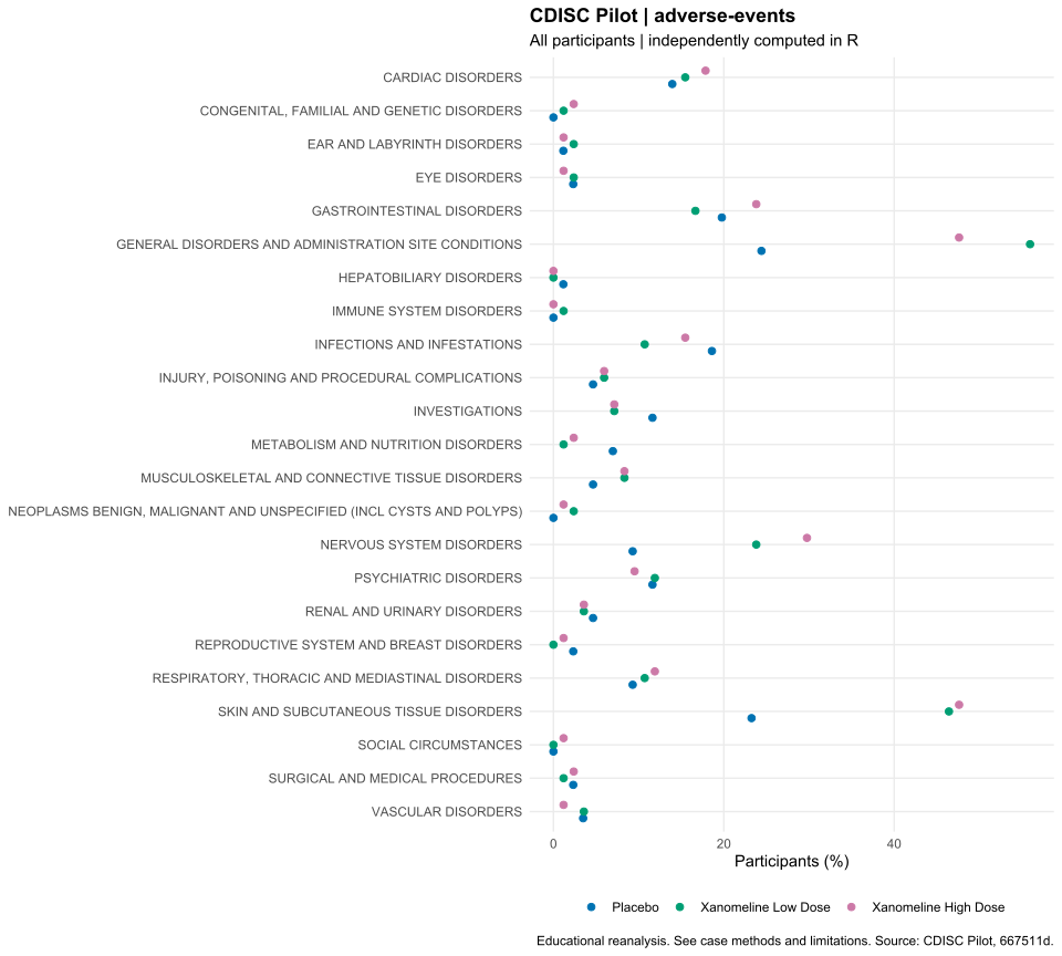
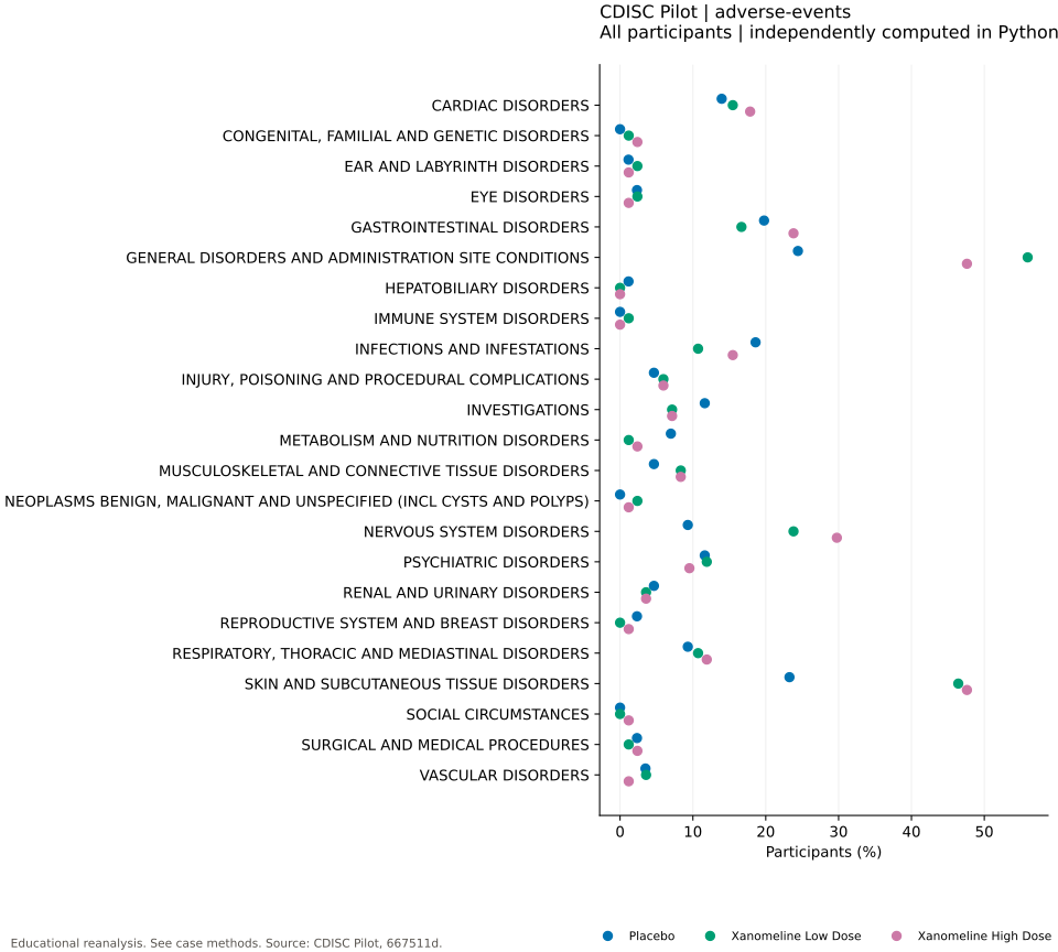
Figures rendered by R and Python
Separately rendered SVG exports from each language's own results. These downloads always use all participants and the original single-measure display (baseline: age; AE: SOC); they do not follow browser filters. These original analysis exports retain their original layout and palette. For the redesigned current view, use Download chart above.
Data
The population behind the result
ADSL safety population, actual treatment; ADAE records with TRTEMFL = Y.
- Dataset and variables
- ADAE: USUBJID, TRTEMFL, AEBODSYS (SOC), AEDECOD (PT). Denominator comes from ADSL, including subjects with no event.
- Source
- CDISC SDTM/ADaM Pilot Project, commit
667511d. Public test data; no employer data or additional synthetic endpoints. Original XPT files are downloaded unchanged and kept outside public assets.
Provenance, dictionary and source terms · Download full case results (JSON, all strata)
Methods
What was estimated—and what was not
Within each SOC or SOC/PT pair, count each subject once for incidence; count all qualifying records separately as events. Any-AE, SOC and PT levels are selectable. Filtering terms changes displayed rows, not the population denominator.
Missing values
No imputation. Subjects without an event remain in the denominator. Empty groups have zero subjects/events. Source dictionary coding is retained; no attempt to recode to a newer dictionary.
Interpretation limits
SOC/PT rows overlap and must not be added to estimate unique subjects. Incidence is not exposure-adjusted and is not evidence of causality.
Display rounding: figure means/percentages 1 decimal, forest contrasts 2 decimals; detail tables up to 3 decimals; counts are integers. Exports retain unrounded numeric results. Sex filters select separately calculated strata. Treatment toggles only select arm-specific results and never recalculate a pooled result.
Quality control
Evidence you can inspect
Independent R and Python outputs agree for this case, including counts, denominators, estimates and available intervals.
Tool identity / permitted local entry point is pending confirmation. Numerical agreement is not a package risk assessment.
Absolute and relative tolerance: 1e-9. Executed: . Counts are checked without rounding; known-answer mean, SD and tied-event/censor fixtures run in both languages.
Reproduce
From unchanged input to checked output
Download the files below into one directory. Use the recorded R/Python package versions; no package is installed by these scripts. The data download contacts only the public source repository. Both analysis scripts run without network access.
python fetch-data.py
Rscript --vanilla analyze.R inputs outputs/r
python analyze.py inputs outputs/python
Data fetch script · R analysis · Python analysis · Environment and hashes · Input SHA-256 manifest
The full local project also includes tools/clinical-data-lab/verify.py for fail-closed comparison and export. No random seed is needed: all analyses are deterministic.